Designing Fair Multiple Choice Tests

A friend of mine scored a 90% on a pretty hard 120 question multiple choice exam that we took and jokingly remarked that he got lucky. Did he though?

Given that he actually knows 90% of the material, what should his test score distribution look like? Assume there are $n$ questions on the test and he has a probability $p$ of being correct on each question. We simulate this by drawing $n$ times from a binomial with success probability $p$. Let $Y \sim binomial(n, p)$ with $E(Y) = np$ and $V(Y) = np(1-p)$. The normal distribution with mean $np$ and variance $np(1-p)$ is an approximation for the binomial and converges as $n$ increases. But, for small $n$, it does not capture the behavior.

library(tidyverse)

#number of questions on test
n <- c(10, 25, 50, 75, 100, 125, 150, 175, 200, 225, 250, 300)

#prob of getting question correct
p <- 0.9

n.samples <- 10000
get_samples <- function(n, p, n.samples){
	y <- rbinom(n=n.samples, size = n, prob = p )

	data.frame(y=y, percent=round((y*100)/n, 2), n=n) %>% as_tibble()
}


data <- do.call(rbind, lapply(n, function(w) get_samples(w, p, n.samples)))

data %>% ggplot(aes(y=percent, x=n, group=n)) + geom_boxplot(color="black", fill="grey70", alpha=0.7, outlier.alpha = 0) + theme_minimal() + xlab("Number of Questions on Test") + ylab("Percentage on Test")  + theme(axis.text=element_text(size=12), axis.title=element_text(size=18), panel.grid = element_blank(), panel.border = element_rect(color="black", fill="transparent")) + geom_hline(yintercept=p*100, color="black", lty="dashed") + scale_y_continuous(n.breaks=10)

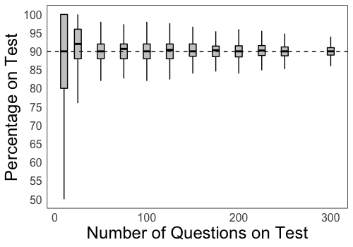
Notice that as the number of questions on the test increases, the score distribution gets tighter. This is an expected result.

But, by how much does the variance in outcomes decrease as a function of the number of questions? If we understand this, we can possibly find the minimum number of questions to have on a multiple choice test to truly capture the knowledge profile of the test taker.

It seems reasonable that most of the time we should want the test taker to score within 5% of his true knowledge. Specifically, if the student knows 80% of the material, we should design a test such that 90% of the time the student scores between a 75% and 85%. What is the minimum number of questions we must ask such that this condition is satisfied for a wide range of knowledge profiles (0-100%)?

We can consider tests with different numbers of questions (e.g., 10, 25, 50 …, 300). We can consider performers of various abilities from those who score 0% to those that score 95%. For each distinct test length and score, we draw from a binomial with parameters defined by these values and do this 10,000 times to simulate the number of questions answered correctly across 10,000 tests. Then, we can figure out if, across these 10,000 performances, the student with true score level $p$ scored within 5 percentage points above or below $p$. The code to do this is shown below:

library(tidyverse)

get_90_outcome_quantile <- function(p){

	n <- c(10, 25, 50, 75, 100, 125, 150, 175, 200, 225, 250, 300)

	n.samples <- 10000
	get_samples <- function(n, p, n.samples){
		y <- rbinom(n=n.samples, size = n, prob = p )

		data.frame(y=y, percent=round((y*100)/n, 2), n=n) %>% as_tibble()
	}

	data <- do.call(rbind, lapply(n, function(w) get_samples(w, p, n.samples)))

	data %>% group_by(n) %>% summarize(lb = quantile(percent, 0.05, na.rm=T), ub = quantile(percent, 0.95, na.rm=T)) %>% mutate(p = p*100) %>% mutate(check = ifelse((lb >= p-5) & (ub <= p+5), "yes", "no")) %>% select(n, p, check)
}

prob.correct <- c(0, .25, .50, .60, .70, .80, .90, .95)

outcomes <- do.call(rbind, lapply(prob.correct, function(x) get_90_outcome_quantile(x)))

ggplot(outcomes, aes(x = factor(p), y = factor(n), fill = check)) + geom_tile(color="black")  + scale_fill_manual(values = c("yes" = "maroon", "no" = "navy"), labels=c("yes" = "outcome within\n5% of knowledge level 90% of the time", "no"="outcome not within\n5% of knowledge level 90% of the time")) + labs(x = "Percent of Material Student Knows", y = "Number of Test Questions", fill = "") + theme_minimal()

A fair test should have a total number of questions such that for each student score level, 90% of the time the performances lie within 5% of that level. Essentially, in the figure below, a row with all maroon squares implies that a test of that question length is fair.

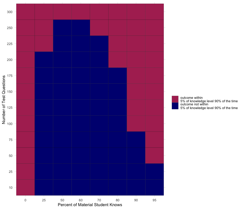
Tests with 300 questions are the only fair length. None of the other questions lengths was able to confine student performance within 5% of their true knowledge level in 90% or more of cases. But, we may be being too restrictive with our criteria. Do we really care that someone who knows 25% of the material scores between 20-30% most of the time? Typically, scores below a 60% are given a fail grade. So, for true knowledge levels less than 60%, we can revise our condition to be “90% of the time the student should score less than the maximum of 60% and their true knowledge level plus 5%”. We adjust the code chunk above replacing get_90_outcome_quantile with the below eval_outcome_distr and arrive at the following result.

eval_outcome_distr <- function(p){

	n <- c(10, 25, 50, 75, 100, 125, 150, 175, 200, 225, 250, 300)

	n.samples <- 10000
	get_samples <- function(n, p, n.samples){
		y <- rbinom(n=n.samples, size = n, prob = p )

		data.frame(y=y, percent=round((y*100)/n, 2), n=n) %>% as_tibble()
	}

	data <- do.call(rbind, lapply(n, function(w) get_samples(w, p, n.samples)))

	adjust_below_60 <- function(x){

		if (quantile(x, 0.95, na.rm=T) <= 60){
			return("yes")
		} else{
			return("no")
		}

	}

	data %>% group_by(n) %>% summarize(lb = quantile(percent, 0.05, na.rm=T), ub = quantile(percent, 0.95, na.rm=T), check_below_60=adjust_below_60(percent)) %>% mutate(p = p*100) %>% mutate(check = ifelse((lb >= p-5) & (ub <= p+5), "yes", "no")) %>% mutate(check = ifelse(p < 60, check_below_60, check)) %>% select(n, p, check)
}

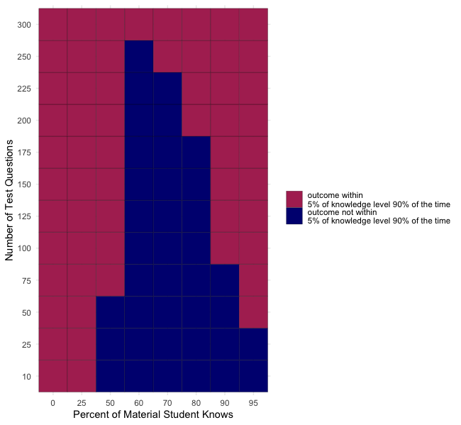
Now, for the squares that are still navy, let us understand the distribution of outcomes in this boxes. What is the 5th and 95th percentile of the data in each navy box? And how close are those observed values to the 5% window we are aiming for? We swap out eval_outcome_distr for investigate_distr, run the code to get the outcomes dataframe.

investigate_distr <- function(p){

	n <- c(10, 25, 50, 75, 100, 125, 150, 175, 200, 225, 250, 300)

	n.samples <- 10000
	get_samples <- function(n, p, n.samples){
		y <- rbinom(n=n.samples, size = n, prob = p )

		data.frame(y=y, percent=round((y*100)/n, 2), n=n) %>% as_tibble()
	}

	data <- do.call(rbind, lapply(n, function(w) get_samples(w, p, n.samples)))

	report_quantile <- function(x, y){

		t <- quantile(x, probs=seq(0.01, 0.99, 0.01))

		names(t)[which.min(abs(t - y))]
	}

	data %>% group_by(n) %>% summarize(lb = quantile(percent, 0.05, na.rm=T), ub = quantile(percent, 0.95, na.rm=T), l5=report_quantile(percent, p*100 - 5), u5=report_quantile(percent, p*100 + 5)) %>% mutate(p = p*100) %>% mutate(check = ifelse((lb >= p-5) & (ub <= p+5), "yes", "no")) %>% select(n, p, check, lb, ub, l5, u5)
}

Now, we plot our data:

df <- outcomes %>% filter(n >= 75, p >= 60, n < 300,check=="no") %>% select(-check) %>% mutate(l5=gsub("%", "", l5) %>% as.numeric(), u5=gsub("%", "", u5) %>% as.numeric(), pup=p+5, pdown=p-5) %>% pivot_longer(-c(n,p), names_to="var", values_to="val") %>% mutate(var=case_when(var=="lb"~"emp", var=="ub"~"emp", var=="pup"~"p", var=="pdown"~"p", var=="u5"~"percentile", var=="l5"~"percentile")) %>% filter(var %in% c("emp", "p")) %>% mutate(plab = paste0(n, " Question\nTest") %>% factor()) 

levels(df$plab) <- c(tail(levels(df$plab), n=1), levels(df$plab)[1:length(levels(df$plab))-1])

df %>% ggplot(aes(x=factor(p), y=val, color=var)) + geom_point(position=position_dodge(width=0.5)) + geom_line(position=position_dodge(width=0.5)) + theme_minimal() + facet_wrap(~plab, scales="free_x", nrow=1) + ylab("Percentage Score Student\nScores on Test") + xlab("Knowledge Level of Student (% of content they actually know)") + scale_color_manual(name="", labels=c("emp"="Observed 5th and 95th percentile", "p"="Expected 5% Window"), values=c("#006400","#FFA500")) + theme(panel.grid=element_blank(), panel.border = element_rect(color="black", fill="transparent")) + theme(legend.position="bottom") + ggtitle("Empirical 90% Intervals For Cases Where Tests Lengths\nLead To Performance Outside 5% Windows More Than 10% of the Time") + geom_hline(yintercept=seq(floor(min(df$val/10))*10, ceiling(max(df$val/10))*10, 2.5), linetype="dashed", color="grey70", alpha=0.8)

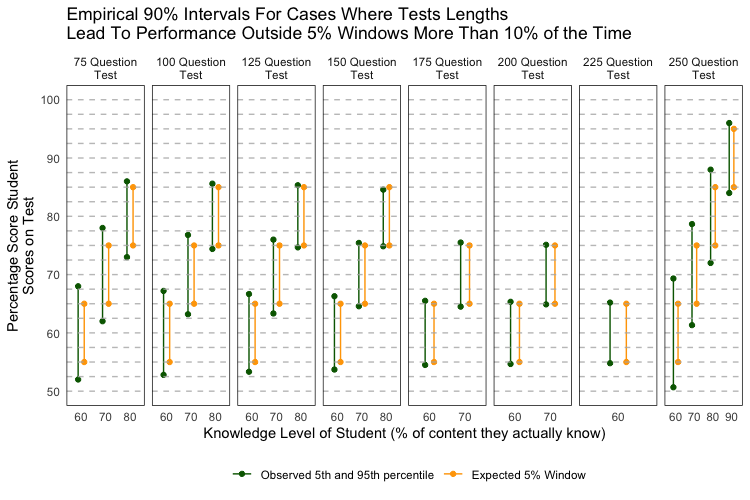
We only look at tests that are sufficiently long (>= 75 questions) but not too long (<300 questions) and boxes that are “navy” or do not have outcomes 90% of time within the target 5% performance window. Each grey horizontal line in the figure correpsonds to 2.5%. Notice that the empirical 90% intervals (dark green lines) are within 2.5% windows of the target ranges (yellow lines) across most test sizes. Specifically the empirical intervals are very tight (mostly within 1%) of the targets for tests with 100-175 questions. We can accept this divergence from our key decision rule.

Based on these analyses, tests with 100 multiple choice questions are the minimum number of questions necessary to ensure that students almost always (>= 90% of the time) score within 5-6% of their true knowledge status.

Tests longer than this are most likely also fair. The MCAT is 230 questions long which is fair by our criteria but the sheer length of the test requires that we factor in mental stamina and the time that someone can remain focused while performing at a level equal to their true knowledge profile. For example, at the beginning of a long test when you are fresh it is easy to perform to the level at which you are prepared. But, as the test wanes on and you become fatigued, your performance may drop even though your actual knowledge status will not have. We did not model this mental stamina component here, so our simulation results of ultra-long (>200 questions) tests may not be entirely valid. Another overarching limitation is that we assume that for a given student, the probability of getting a question correct is independent of the prior questions. Accounting for dependence will allow us to create more representative models.