Streaming computation of statistical measures

Suppose I have a stream of numbers being fed into a computer. The stream is of finite length, but very large, and I am interest in calculating some statistical properties of the stream at each length $l$.

Why is this relevant? For example, this could be Apple Watch sensor data reporting the HR of the user every minute. I have HR data from the past and want to update HR stats (e.g., mean, variance, median) when the next HR timepoint comes in.

TL;DR: Mean and variance are easy to compute in a streaming fashion, see below. Median and other higher order moments, not so much, but some streaming algorithms approximate them well. I wonder how the Apple Watch team computes the running median without storing all the data? With enough samples, assuming the law of large numbers holds, the mean coincides with the median. In generla, the mean approximate the median decently as the number of samples increases. If not, a correction using the variance or some other calculable moment can probably approximate the median well enough. Also, this setup we are considering of never storing data is contrived.

Ok, let’s consider the non-streaming way to compute statistical measures on data. We store the raw data points $x_1, x_2, … , x_n$ and then when $x_{n+1}$ arrives, use the entire sequence to compute the properties of interest (e.g., variance, mean, skewness). This is inefficient because it requires that we store all the data and that we loop over the entire data stream whenever new data arrives. These two operations get increasingly costly as the number of data points increases.

We would like to compute our statistical measure of interest while throwing out data $x_i$ as we see them such that there is only the most recent data point in storage.

Let us derive an expression for the mean, $\bar{x}$. Note that, by definition, $\bar{x} = \frac{1}{n} \sum_{i=1}^{n} x_i$. We can compute the mean by keeping track of two numbers: the running sum $s_n$ where $s_1 = x_1$, $s_2 = s_1 + x_2$, and so forth; $n$ which is incremented by one every time we update $s_n$. Doing $\frac{s_n}{n}$ gives us $\bar{x}$. There is another way to compute the mean iteratively. Note that $\bar{x_n} = \frac{x_1 + … + x_n}{n}$ and $\bar{x_{n+1}} = \frac{x_1 + … + x_n + x_{n+1}}{n+1}$. From the former expresion, $(x_1 + … + x_n) = n \cdot \bar{x_n}$ and therefore $\bar{x_{n+1}} = \frac{n \cdot \bar{x_n} + x_{n+1}}{n+1}$ which means $\bar{x_{n+1}} = \frac{n}{n+1}\bar{x_n} + \frac{x_{n+1}}{n+1}$. The base case is that $\bar{x_1} = x_1$ and from there we keep track of $\bar{x_n}$ and increment $n$ by one every time we compute $\bar{x_n}$. These methods are essentially equivalent in terms of complexity and memory though.

Let us derive an iterative expression for the sample variance, $V(x_n) = \frac{\sum_{i=1}^{n} (x_i - \bar{x_n})^2 }{n-1}$. As is, this cannot be computed iteratively because we have $x_i$ tied to $x_n$ which means reupdating the difference for each previous value based on the new mean. Let us expand this square and distribute the sum operator and see where that takes us.

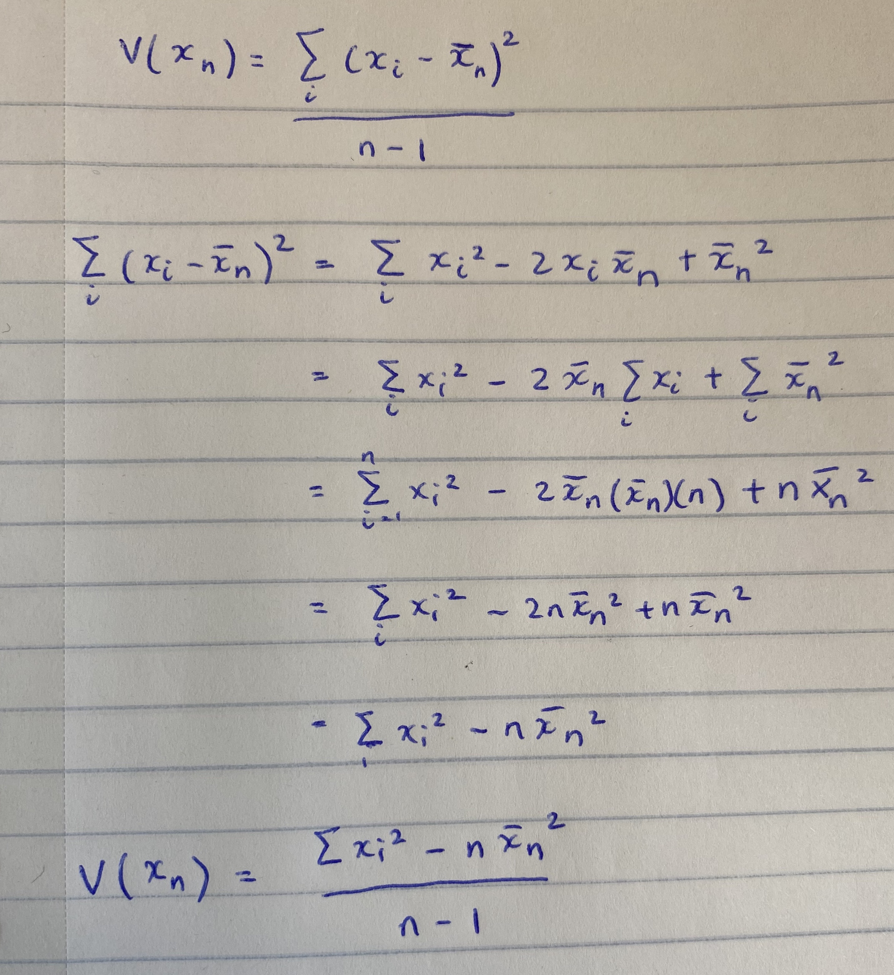
Decomposition of sample variance

We need to track three things to compute sample variance without storing the stream of data: a) $\Omega$, Sum of Squares of Individual data points, b) the mean (which we already have), c) $n$, which we already have from computing the mean. The $\Omega_{n_1} = \Omega_{n} + x_{n+1}^2$ with base case $\Omega_1 = x_1^2$.

Can we compute the median without storing the stream of numbers? The median of a set is the 50th percentile of the set - sort the numbers and find the middle value. One solution would be to set up $p$ bins. Then as the data $x_i$ arrive, do binary sort to find the bin $x_i$ belongs to and increment the count of that. This way, after observing $n$ data values, we have only stored $p$ values and can compute the median from the histogram bins. The accuracy of our median estimate is limited by our choice of bin size. As bin size decreases, median accuracy increases but so too does storage cost. Note that binary sort for each value takes O(log p) where $p$ is the number of bins we define. It does not run in constant time so we give up time to save on space.

The $P^2$ algorithm for dynamic calculcation of quantiles and histograms without sorting observations is a cool paper from over 30 years ago that computes running medians with mean-squared error that quickly asymptotes to zero as the number of observations increases. We can see this relationship when the data comes from an exponential and normal distribution, respectively.

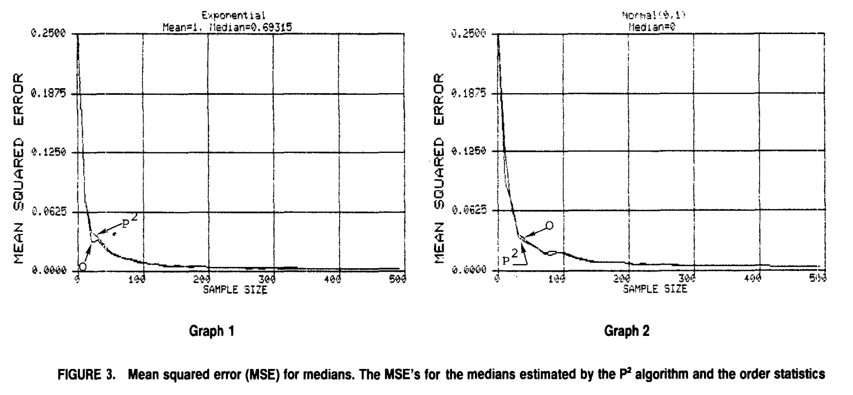
Does this mean-squared error drop off extend for non-standard distributions like the Cauchy? This is irrelevant in my opinion. With large enough sample size, as in the case we consider here, everything basically resembles a Gaussian or a mixture of Gaussians. The real question is whether this algorithm works for the mixture case.

What is the $P^2$ algorithm?

The algorithm consists of maintaining five markers: the minimum, the p/2-, p-, and (1 + p)/2 quantiles, and the maximum. The markers are numbered 1-5 or equivalently $q_1$ to $q_5$. Markers 2 and 4 are also called middle markers because they are midway between the p-quantile (marker 3) and the extremes. As shown in Figure 2 (which is a rotated version of Figure 1), the vertical height of each marker is equal to the corresponding quantile value, and its horizontal location is equal to the number of observations that are less than or equal to the marker. True values of the quantiles are, obviously, not known; at any point in time, the marker heights are the current estimates of the quantiles, and these estimates are updated after every observation.

The pseudo-code provided in the paper is quite clear and easy to follow. The five markers are updated with each new data point. An ideal marker location is also computed and if a marker is located off the ideal by more than one, then the value (height) and location of the marker is updated piecewise parabolic prediction (PP or $P^2$) formula. The formula assumes that the curve passing through any three adjacent markers is a parabola of the form $q_i = a \cdot n_i^2 + b \cdot n_i + c$ and the exact equation can be found in the main text of the paper. It would be interesting to implement this algorithm, then draw samples from a mixture of Gaussians and plot the relationship between MSE and sample size. One could start with a mixture of 2 gaussians with equal weights and different means and variances and recreate figure 3 of the Jain paper.